
Do you want to represent and understand complex data? The best way to do it will be by using heatmaps. Heatmap is a data visualization technique, which represents data using different colours in two dimensions. In Python, we can create a heatmap using matplotlib and seaborn library. Although there is no direct method using which we can create heatmaps using matplotlib, we can use the matplotlib imshow function to create heatmaps.
In a Matplotlib heatmap, every value (every cell of a matrix) is represented by a different color. Data Scientists generally use heatmaps when they want to understand the correlation between various features of a data frame. If you are unaware of all these terms, don’t worry, you will get a basic idea about it when discussing its implementation.
Syntax of Matplotlib Heatmap
To generate a heatmap using matplotlib, we will use the imshow function of matplotlib.pyplot and two of its parameters – ‘interpolation’ and ‘cmap.’ Let us understand these parameters.
Before that, you need to install matplotlib library in your systems if you have not already installed. You need to use this command – pip install matplotlib.
imshow(data, cmap=None,interpolation=None)
Parameters-
- Data – In this data parameter, we have to pass a 2D array as an input.
- Cmap– Using this parameter, we can give colour to our graph. We can choose the colour from the below options.
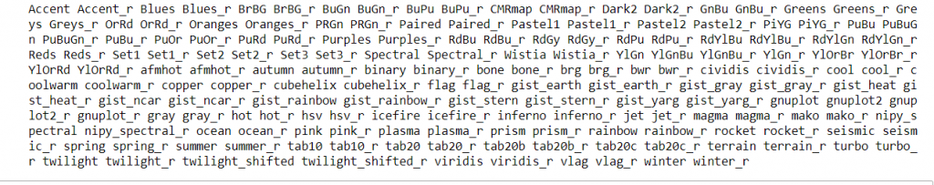
- Interpolation – Different types of graphs can be created. We can choose any of the following values and fill in the interpolation parameter.
antialiased, none, nearest, bilinear, bicubic, spline16, spline36, hanning, hamming, hermite, kaiser, quadric, catrom, gaussian, bessel, mitchell, sinc, lanczos, blackman
Return Type
<class ‘matplotlib.image.AxesImage’>
Heatmaps using Matplotlib
Creating our First Heatmap using matplotlib
Suppose we have marks obtained by different students in different subjects out of 100. Let us see how we can use heatmaps to represent this data.
import matplotlib.pyplot as plt

# Create a array of marks in different subjects scored by different students
marks = np.array([[50, 74, 40, 59,90, 98],
                    [72, 85, 64, 33, 47, 87],
                    [52, 97, 44, 73, 17, 56],
                    [69, 45, 89, 79,70, 48],
                    [87, 65, 56, 86, 72, 68],
                    [90, 29, 78, 66, 50, 32]])
# name of students
names=['Sumit','Ashu','Sonu','Kajal','Kavita','Naman']
# name of subjects
subjects=['Maths','Hindi','English','Social Studies','Science','Computer Science']

# Setting the labels of x axis.
# set the xticks as student-names
# rotate the labels by 90 degree to fit the names
plt.xticks(ticks=np.arange(len(names)),labels=names,rotation=90)
# Setting the labels of y axis.
# set the xticks as subject-names
plt.yticks(ticks=np.arange(len(subjects)),labels=subjects)
# use the imshow function to generate a heatmap
# cmap parameter gives color to the graph
# setting the interpolation will lead to different types of graphs
plt.imshow(marks, cmap='cool',interpolation="nearest")
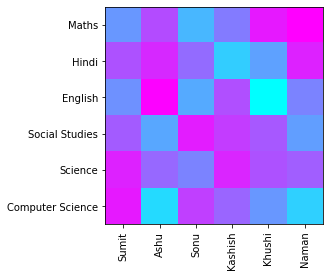
In the above heatmap, dark colors show good marks, and light color shows bad marks. Heatmaps adjust the brightness of the color according to the highest and lowest marks in the dataset. The highest score is represented by the darkest color and the lowest score by the brightest color.
Playing with interpolation and cmap parameters
Let us now change the cmap and interpolation on the same data and see what are the varieties of graphs we can make.
import matplotlib.pyplot as plt
marks = np.array([[50, 74, 40, 59,90, 98],
                    [72, 85, 64, 33, 47, 87],
                    [52, 97, 44, 73, 17, 56],
                    [69, 45, 89, 79,70, 48],
                    [87, 65, 56, 86, 72, 68],
                    [90, 29, 78, 66, 50, 32]])

names=['Sumit','Ashu','Sonu','Kajal','Kavita','Naman']
subjects=['Maths','Hindi','English','Social Studies','Science','Computer Science']

plt.xticks(ticks=np.arange(len(names)),labels=names,rotation=90)
plt.yticks(ticks=np.arange(len(subjects)),labels=subjects)
# set the cmap as Blues and interpolation as spline16
plt.imshow(marks, cmap='Blues',interpolation="spline16")
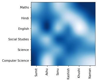
In this graph whenever the marks are more, the color is quite dark, and where the score is less, the color is lighter.
Adding Colorbar in Heatmap using Matplotlib
Colorbar can simply be understood as a scale that helps us understand which color represents which value. Also, there is a direct function in matplotlib for adding a color bar to the graph. Let us use the same data as above for this purpose.
import matplotlib.pyplot as plt
marks = np.array([[50, 74, 40, 59,90, 98],
                    [72, 85, 64, 33, 47, 87],
                    [52, 97, 44, 73, 17, 56],
                    [69, 45, 89, 79,70, 48],
                    [87, 65, 56, 86, 72, 68],
                    [90, 29, 78, 66, 50, 32]])

names=['Sumit','Ashu','Sonu','Kajal','Kavita','Naman']
subjects=['Maths','Hindi','English','Social Studies','Science','Computer Science']

plt.xticks(ticks=np.arange(len(names)),labels=names,rotation=90)
plt.yticks(ticks=np.arange(len(subjects)),labels=subjects)
# save this plot inside a variable called hm
hm=plt.imshow(marks, cmap='Blues',interpolation="nearest")
# pass this heatmap object into plt.colorbar method.
plt.colorbar(hm)
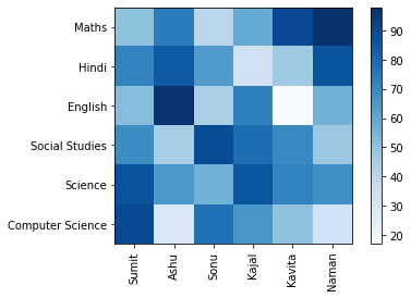
You can see a vertical line around the heatmap. This is a color bar. It clearly indicates that, for higher marks, the color is dark and for lower marks, the color is a lighter shade.
Correlation Between Features in Pandas Dataframe using matplotlib Heatmap
One of the greatest applications of the heatmap is to analyze the correlation between different features of a data frame. Features mean columns and correlation is how much values in these columns are related to each other.
Let us take a data frame and analyze the correlation between its features using a heatmap.
import pandas as pd
import matplotlib.pyplot as plt

# this is our data
x=[[1.,337.,118.,4.,4.5 ,4.5 ,9.65,1.,0.92],[2.,324.,107.,4.,4.,4.5 ,8.87,1.,0.76],[3.,316.,104.,3.,3.,3.5 ,8.,1.,0.72],
[4.,322.,110.,3.,3.5 ,2.5 ,8.67,1.,0.8 ],[5.,314.,103.,2.,2.,3.,8.21,0.,0.65],[6.,330.,115.,5.,4.5 ,3.,9.34,1.,0.9 ],
[7.,321.,109.,3.,3.,4.,8.2 ,1.,0.75],[8.,308.,101.,2.,3.,4.,7.9 ,0.,0.68],[9.,302.,102.,1.,2.,1.5 ,8.,0.,0.5 ],
[ 10.,323.,108.,3.,3.5 ,3.,8.6 ,0.,0.45],[ 11.,325.,106.,3.,3.5 ,4.,8.4 ,1.,0.52],[ 12.,327.,111.,4.,4.,4.5 ,9.,1.,0.84],
[ 13.,328.,112.,4.,4.,4.5 ,9.1 ,1.,0.78],[ 14.,307.,109.,3.,4.,3.,8.,1.,0.62],[ 15.,311.,104.,3.,3.5 ,2.,8.2 ,1.,0.61],
[ 16.,314.,105.,3.,3.5 ,2.5 ,8.3 ,0.,0.54],[ 17.,317.,107.,3.,4.,3.,8.7 ,0.,0.66],[ 18.,319.,106.,3.,4.,3.,8.,1.,0.65],
[ 19.,318.,110.,3.,4.,3.,8.8 ,0.,0.63],[ 20.,303.,102.,3.,3.5 ,3.,8.5 ,0.,0.62],[ 21.,312.,107.,3.,3.,2.,7.9 ,1.,0.64],
[ 22.,325.,114.,4.,3.,2.,8.4 ,0.,0.7 ],[ 23.,328.,116.,5.,5.,5.,9.5 ,1.,0.94],[ 24.,334.,119.,5.,5.,4.5 ,9.7 ,1.,0.95],
[ 25.,336.,119.,5.,4.,3.5 ,9.8 ,1.,0.97],[ 26.,340.,120.,5.,4.5 ,4.5 ,9.6 ,1.,0.94],
[ 27.,322.,109.,5.,4.5 ,3.5 ,8.8 ,0.,0.76],[ 28.,298.,98.,2.,1.5 ,2.5 ,7.5 ,1.,0.44],[ 29.,295.,93.,1.,2.,2.,7.2 ,0.,0.46],
[ 30.,310.,99.,2.,1.5 ,2.,7.3 ,0.,0.54],[ 31.,300.,97.,2.,3.,3.,8.1 ,1.,0.65],
[ 32.,327.,103.,3.,4.,4.,8.3 ,1.,0.74], [ 33.,338.,118.,4.,3.,4.5 ,9.4 ,1.,0.91], [ 34.,340.,114.,5.,4.,4.,9.6 ,1.,0.9 ],
[ 35.,331.,112.,5.,4.,5.,9.8 ,1.,0.94], [ 36.,320.,110.,5.,5.,5.,9.2 ,1.,0.88],
[ 37.,299.,106.,2.,4.,4.,8.4 ,0.,0.64], [ 38.,300.,105.,1.,1.,2.,7.8 ,0.,0.58], [ 39.,304.,105.,1.,3.,1.5 ,7.5 ,0.,0.52],
[ 40.,307.,108.,2.,4.,3.5 ,7.7 ,0.,0.48], [ 41.,308.,110.,3.,3.5 ,3.,8.,1.,0.46], [ 42.,316.,105.,2.,2.5 ,2.5 ,8.2 ,1.,0.49],
[ 43.,313.,107.,2.,2.5 ,2.,8.5 ,1.,0.53], [ 44.,332.,117.,4.,4.5 ,4.,9.1 ,0.,0.87], [ 45.,326.,113.,5.,4.5 ,4.,9.4 ,1.,0.91],
[ 46.,322.,110.,5.,5.,4.,9.1 ,1.,0.88], [ 47.,329.,114.,5.,4.,5.,9.3 ,1.,0.86], [ 48.,339.,119.,5.,4.5 ,4.,9.7 ,0.,0.89],
[ 49.,321.,110.,3.,3.5 ,5.,8.85,1.,0.82], [ 50.,327.,111.,4.,3.,4.,8.4 ,1.,0.78]]

# column name
columns=['Serial No.', 'GRE Score', 'TOEFL Score', 'University Rating', 'SOP',
       'LOR ', 'CGPA', 'Research', 'Chance of Admit ']

# create a dataframe with the above values and column names
dataset=pd.DataFrame(data=x,columns=columns)

# to find the correlation, use corr() method on the dataset
corr=dataset.corr()

plt.xticks(range(len(columns)),columns,rotation=90)
plt.yticks(range(len(columns)),columns)
plt.imshow(corr, cmap='hot',interpolation="nearest")
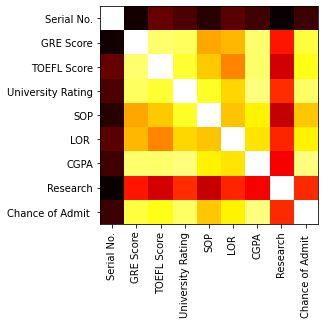
In the above heatmap, the lighter the value, the more the correlation between the features. You can see that if we want to check which features are more correlated to the Chance of Admit, you will see the following row-
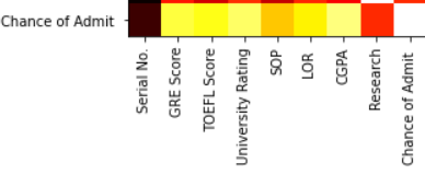
Notice that for higher Chance of admission, CGPA and University matters the most because they have very bright colors. Also, Serial No. and research don’t matter that much. This is how we take advantage of heatmaps in data science.
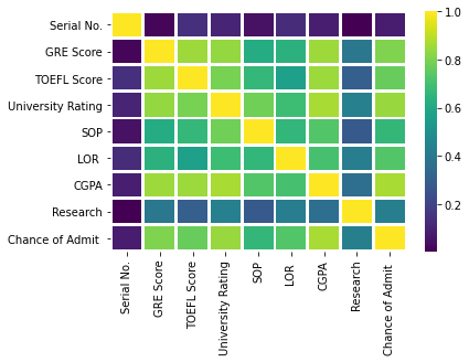
Heatmaps using Seaborn
Seaborn is a data visualization library that is built on top of matplotlib and contains a direct function to create heatmaps. Before using seaborn, install it in your systems using pip install seaborn.
We will use the above data to see how seaborn heatmaps can be created.
# import the seaborn library and give alias as sns
import seaborn as sns
# use heatmap function, set the color as viridis and
# make each cell seperate using linewidth parameter
sns.heatmap(corr,linewidths=2,cmap="viridis")
Must Read:
- How to Convert String to Lowercase in
- How to Calculate Square Root
- User Input | Input () Function | Keyboard Input
- Best Book to Learn Python
Conclusion
To analyse and visualize data in a better way, we can use heatmaps. To create heatmaps using matplotlib, we need to use imshow function with cmap and interpolation parameters. Data Scientist generally use heatmaps for analysing the correlation between different features of a dataset.