
Quick answer: np.cov estimates covariance and returns a covariance matrix. Decide whether rows or columns represent variables with rowvar, keep paired observations aligned, and distinguish covariance’s original units from correlation’s normalized scale.
NumPy cov() calculates covariance from one or more variables. Covariance describes how two variables move together: positive covariance means they tend to increase together, negative covariance means one tends to increase while the other decreases, and a value near zero means the linear movement is weak.
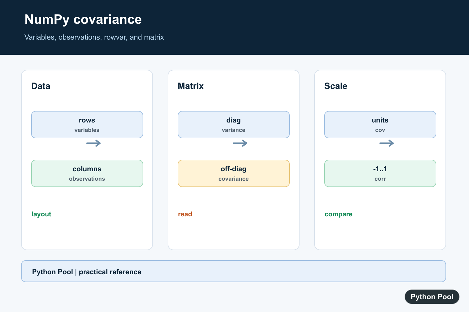
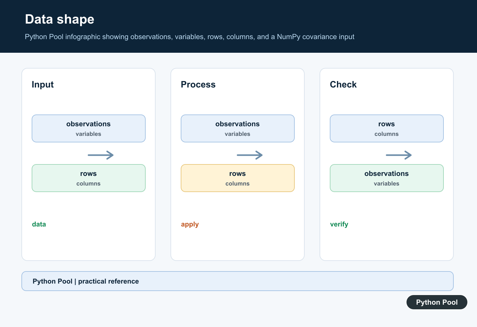
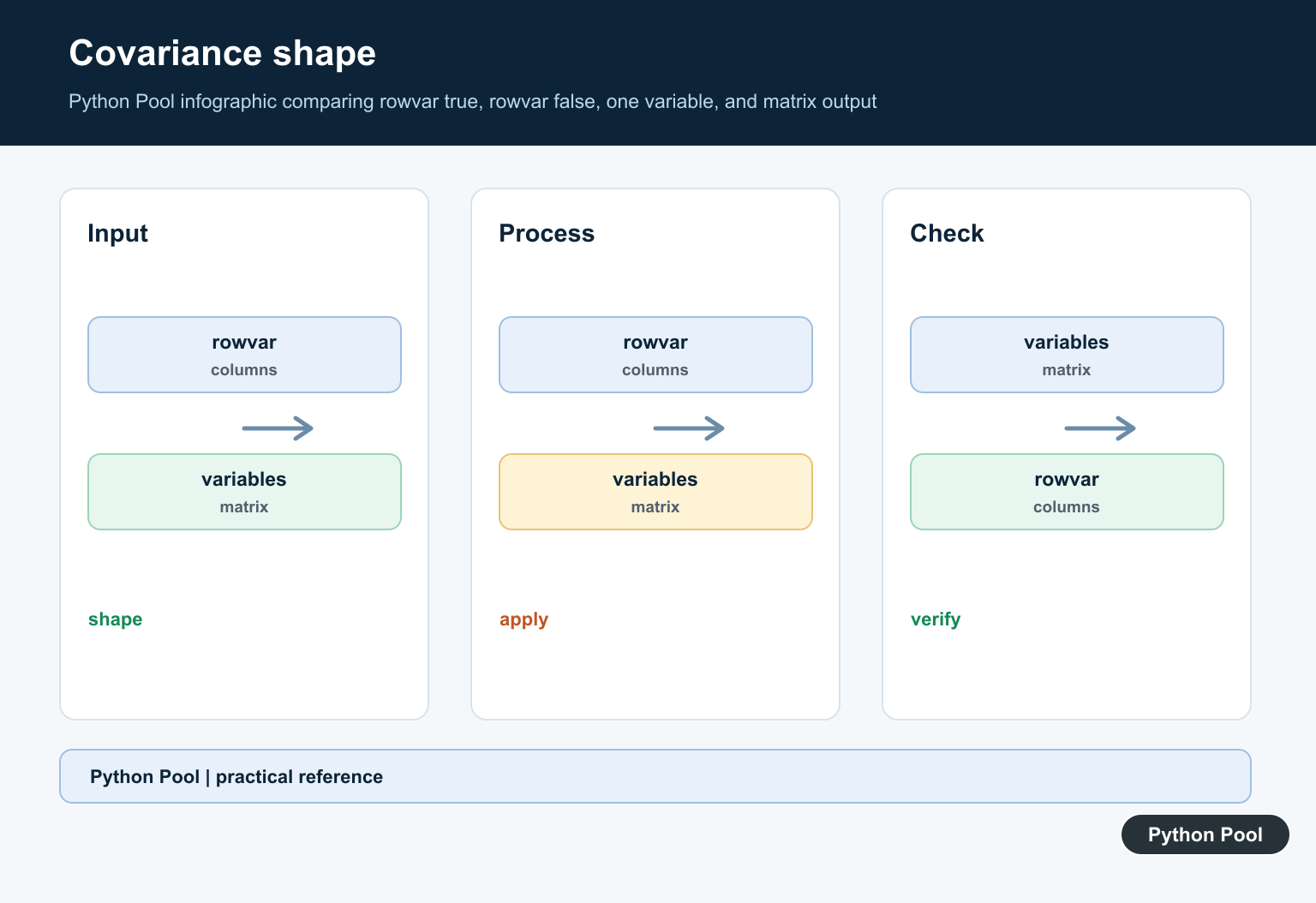
The function returns a covariance matrix. For two variables, the diagonal cells are variances and the off-diagonal cells are covariances. The most common source of confusion is array shape: by default, NumPy treats each row as a variable and each column as an observation. Use rowvar=False when your columns are variables.
Covariance is not the same as correlation. Covariance keeps the units of the original data, while correlation is scaled to a range from -1 to 1. Use covariance when units matter and correlation when you need a normalized relationship strength.
Before calculating covariance, make sure paired observations line up correctly. If the first value in x belongs with the first value in y, filtering, sorting, or reshaping one array without the other can make the output meaningless.
Calculate Covariance Between Two Lists
The official numpy.cov() function accepts two one-dimensional arrays or lists. Passing two variables returns a 2 by 2 matrix.
import numpy as np

x = [2, 4, 6, 8]
y = [1, 3, 5, 7]

matrix = np.cov(x, y)
print(matrix)
The top-left value is the variance of x, the bottom-right value is the variance of y, and the off-diagonal values are the covariance between x and y. The matrix is symmetric because the covariance of x with y equals the covariance of y with x.
Use rowvar=False for Column Variables
If your data is shaped like a table, each row is often one observation and each column is one variable. In that case, set rowvar=False so NumPy interprets columns as variables.
import numpy as np

data = np.array([
    [2, 1],
    [4, 3],
    [6, 5],
    [8, 7],
])

matrix = np.cov(data, rowvar=False)
print(matrix)
This is the safer setting for spreadsheet-style data, Pandas-like tables, and machine-learning feature matrices. If a covariance result has an unexpected shape, check rowvar before checking the math. For shape cleanup examples, see NumPy reshape 3D to 2D.
Control Bias and Degrees of Freedom
By default, np.cov() normalizes by N - 1, which gives the sample covariance. You can change the normalization with bias or ddof.
import numpy as np

x = np.array([2, 4, 6, 8])
y = np.array([1, 3, 5, 7])

sample_cov = np.cov(x, y)
population_cov = np.cov(x, y, bias=True)

print(sample_cov)
print(population_cov)
Use the sample version when your data is a sample from a larger population. Use population-style normalization only when the data represents the whole population you want to describe. Being explicit about this choice prevents small but important reporting differences.
Compare Covariance With Correlation
numpy.corrcoef() returns correlation coefficients, not covariance values. It is useful when variables use different units or scales.
import numpy as np

x = np.array([2, 4, 6, 8])
y = np.array([1, 3, 5, 7])

covariance = np.cov(x, y)
correlation = np.corrcoef(x, y)

print(covariance)
print(correlation)
If a variable is measured in dollars and another is measured in seconds, covariance can be hard to compare directly. Correlation helps with comparison, while covariance keeps the original scale. For averaging concepts used in both formulas, see Python average of list and the NumPy mean reference. Covariance describes joint variation, while T Test in Python with SciPy Examples shows how to test whether sample means differ significantly.
Handle Missing Values Before Calling cov()
np.cov() does not automatically ignore arbitrary missing values in plain arrays. Clean or filter the data first so paired observations stay aligned.
import numpy as np

x = np.array([2.0, 4.0, np.nan, 8.0])
y = np.array([1.0, 3.0, 5.0, 7.0])

mask = ~np.isnan(x) & ~np.isnan(y)
matrix = np.cov(x[mask], y[mask])

print(matrix)
The mask keeps only rows where both variables have valid numbers. Filtering one array without filtering the matching positions in the other array changes the pairing and makes the covariance meaningless. This is one reason to clean data in a table-like structure before splitting columns into separate arrays.
Round the Matrix for Display
Covariance matrices often contain floating-point values. Round for presentation, but keep the unrounded matrix for later calculations.
import numpy as np

data = np.array([
    [2, 1, 10],
    [4, 3, 12],
    [6, 5, 14],
    [8, 7, 16],
])

matrix = np.cov(data, rowvar=False)
print(np.round(matrix, 2))
Rounding the displayed output makes examples easier to read. The NumPy round() guide covers related formatting options. If you need to understand vector-style input before covariance, see Python vector with NumPy.
How to Read the Output
Read the covariance matrix by matching row and column positions to your variables. In a three-variable matrix, cell [0, 2] describes the covariance between the first and third variables. The diagonal values are useful too, because they show how much each variable varies by itself. Label the rows and columns in reports so readers do not have to remember the original array order.
Common Mistakes
The most common mistakes are using the wrong rowvar value, comparing covariance values across unrelated units, and forgetting that the diagonal of the matrix contains variances. Always check the shape of the result and label your variables when presenting the matrix.
References
Read The Matrix
The diagonal entries are variances and the off-diagonal entries are pairwise covariances. Positive values indicate variables tend to move together under the chosen data and normalization policy.
Choose rowvar Correctly
By default, each row is treated as a variable and columns are observations. For the common table layout where rows are observations and columns are variables, pass rowvar=False.
Keep Pairs Aligned
Filter, sort, and reshape all variables together. If x[i] no longer corresponds to y[i], the covariance may be mathematically valid for the mispaired arrays but meaningless for the intended relationship.
Compare With Correlation
Covariance carries the units of both variables, so its magnitude depends on scale. Correlation normalizes by standard deviations and is often easier to compare across pairs.
Document Missing Data
Decide whether rows with missing values are removed, imputed, or handled with a masked strategy. The sample size and normalization option affect interpretation, so report them with the matrix.
The NumPy cov reference documents rowvar and covariance output. Related references include variance, axes, and data tests.
For related array statistics, compare variance, axes, and array normalization when interpreting matrix output.
Frequently Asked Questions
What does NumPy cov calculate?
It estimates covariance between variables and returns a covariance matrix.
What does rowvar mean?
With rowvar=True, rows represent variables; use rowvar=False when columns represent variables and rows are observations.
How is covariance different from correlation?
Covariance retains the original units, while correlation normalizes the relationship to a bounded, unit-free scale.
Why must observations stay aligned?
Pairing the wrong x and y observations changes the measured relationship and can make the covariance meaningless.