Working With Python Pywake Library

With the vast amount of python libraries, python does a lot of easy work. Some of its work even automate the calculation and is convenient to use. However, we also need to set our environment as such to get better performance. Some of them are providing good datasets or using good models. These all decide the overall performance of our application. Today, in this article, we will discuss one such library that is the python pywake library. First, we will start with the use of the library. And then, we will set the environment for it and see the demonstration over it. So, let’s begin.

Contents

What is Pywake?

Pywake is a python library used as an AEP calculator for wind farms. It is a simulation tool capable of calculating flow fields or power production for wind farms. Despite being a unified interface of different engineering models, it is very fast in terms of performance. The reason is that developers make heavy use of vectorization and numerical libraries to perform the calculations. Now, once you understand this, let’s go with installation and setting up the environment.

Installation

To install the library, we will use the following command.

pip install py-wake

Setting Up the Environment for Pywake

Once we are done with the installation, we will set the environment for AEP calculation. For that, we will first import the required libraries. Then, we set up wind turbines, site, and flow model. We will do that in the following way.

import py_wake
from py_wake.examples.data.hornsrev1 import Hornsrev1Site,V80, wt_x, wt_y, wt16_x, wt16_y
from py_wake import NOJ

windTurbines = V80()
site=Hornsrev1Site()
noj = NOJ(site,windTurbines)

Calculating AEP

Now, once we initialize the required object, let’s run the model and calculate AEP.

# Running the model
simulationResult = noj(wt16_x,wt16_y)

# Calculating AEP
print ("Total AEP: %f GWh"%simulationResult.aep().sum())
simulationResult.aep()

Plotting AEP

In the above section of the article, we have calculated AEP. Now, it’s time to visualize it on the graph. So, in this section, we will plot the graph of AEP depending on different factors. These factors are wind turbines, wind speed, and wind directions. Let’s plot it.

AEP vs Turbines Plot

import matplotlib.pyplot as plt
%matplotlib inline

plt.figure()
aep = simulationResult.aep()
windTurbines.plot(wt16_x,wt16_y)
c =plt.scatter(wt16_x, wt16_y, c=aep.sum(['wd','ws']))
plt.colorbar(c, label='AEP [GWh]')

In the above image, we have plotted the scattered graph for turbines on the x-axis and AEP on the y-axis. For that, we used the scatter() function, and for the color bar representing AEP, we used the color bar function.

AEP vs Wind Speed Plot

Now, let’s see how AEP varies based on wind speed.

plt.figure()
aep.sum(['wt','wd']).plot()
plt.xlabel("Wind speed [m/s]")
plt.ylabel("AEP [GWh]")

So, in the above example, we can see that the graph’s distribution varies typically along the x-axis. When the wind speed is low or high, the AEP is low. On the other hand, power production is high if it is between 8 to 15.

AEP vs Wind Direction Plot

Now, let’s see how AEP varies depending on the wind direction. We measure direction as the angle here.

plt.figure()
aep.sum(['wt','ws']).plot()
plt.xlabel("Wind direction [deg]")
plt.ylabel("AEP [GWh]")

So, as you can see, AEP is highest when the wind direction is somewhat between 250 to 300 degrees.

So, in this way, we can visualize the energy production in a wind farm using the Pywake library in python.

Setting Up Wind Turbine Object

In the above example, we have seen that we set the wind turbine object using V80 from Hornsrev1, 3.35MW from IEA task 37, and the DTU10MW, a predefined Wind Turbine available in the module. Let’s recap it once.

import os
imprt py_wake
import numpy as np
import matplotlib.pyplot as plt
from py_wake.wind_turbines import WindTurbines
from py_wake.examples.data.hornsrev1 import V80
from py_wake.examples.data.iea37 import IEA37_WindTurbines, IEA37Site
from py_wake.examples.data.dtu10mw import DTU10MW

v80 = V80()
iea37 = IEA37_WindTurbines()
dtu10mw = DTU10MW()

Import from WAsP wtg files

However, we can also import other predefined turbines using WAsP wtg files. After that, we can initialize the wind turbine’s object.

from py_wake.examples.data import wtg_path

wtg = os.path.join(wtg_path, 'NEG-Micon-2750.wtg')
neg2750 = WindTurbines.from_WAsP_wtg(wtg)

User Defined WindTurbine

Besides these predefined classes of wind turbines, we can also create a user-defined wind turbine using the WindTurbine() class. Let’s see how we can do it.

from py_wake.wind_turbines.power_ct_functions import PowerCtTabular
from py_wake.wind_turbines import WindTurbine

initialu = [0,4,12,24,36]
thrust_coeff = [0,0.9,0.8,.3, 0]
power = [0,0,3000,3000,0]

windturbine_obj = WindTurbine(name='MyWT',
                    diameter=124,
                    hub_height=320,
                    powerCtFunction=PowerCtTabular(initialu, power, 'kW', thrust_coeff))

Multi-type Wind Turbines

However, we can also collect a list of different types of wind turbines into a single WindTurbine() object. To do that, we need to pass that list of wind turbines to the constructor of WindTurbine() class as the argument while initializing its object. Let’s see it.

import os
import numpy as np
import matplotlib.pyplot as plt
from py_wake.wind_turbines import WindTurbines
from py_wake.examples.data.hornsrev1 import V80
from py_wake.examples.data.iea37 import IEA37_WindTurbines, IEA37Site
from py_wake.examples.data.dtu10mw import DTU10MW
from py_wake.wind_turbines.generic_wind_turbines import GenericWindTurbine
from py_wake.examples.data import wtg_path

v80 = V80()
iea37 = IEA37_WindTurbines()
dtu10mw = DTU10MW()

u = [0,4,12,24,36]
thrust_coeff = [0,0.9,0.8,.3, 0]
power = [0,0,3000,3000,0]
windturbine_obj = WindTurbine(name='MyWT',
                    diameter=124,
                    hub_height=320,
                    powerCtFunction=PowerCtTabular(u,power,'kW',thrust_coeff))
gen_wt = GenericWindTurbine('G10MW', 180, 120, power_norm=10000, turbulence_intensity=.1)

wts = WindTurbines.from_WindTurbine_lst([v80,iea37,dtu10mw,windturbine_obj,gen_wt])

# To check it
types = wts.types()
print ("Name:\t\t%s" % "\t".join(wts.name(types)))
print('Diameter[m]\t%s' % "\t".join(map(str,wts.diameter(type=types))))
print('Hubheigt[m]\t%s' % "\t".join(map(str,wts.hub_height(type=types))))

Output:

Name:		V80	3.35MW	DTU10MW	MyWT	G10MW
Diameter[m]	80.0	130.0	178.3	124.0	180.0
Hubheigt[m]	70.0	110.0	119.0	320.0	120.0

Engineering Wind Farm Models

While initializing win farm models object, it is necessary to pass a site and a turbine objects as the argument. The engineering windfarm model comprises one wind farm model and one superposition model. One more optional model can be there as blockage deficit and a turbulence model.

WindFarmModel

This model defines the procedure of how the wake and the blockage deficits propagate in the wind farm. Two wind farm models are available for inclusion, i.e., PropagateDownwind and All2Alllternative.

Wake DeficitModel

This is used to calculate the wake deficit from one wind turbine to downstream wind turbines in the wind farm. Several models are available, such as NOJDeficit, TurboNOJDeficit, FugaDeficit, e.t.c.

SuperpositionModel

This model is used, to sum up the deficit from different sources. Available superposition models are LinearSum, SquaredSum, MaxSum.

RotorAvgModel

This model is used to calculate the average rotor deficit from RotorCenter, GridRotorAvg, EqGridRotorAvg e.t.c

DeflectionModel

This model calculates deflected downwind and crosswind distance due to yaw misalignment, shear, e.t.c. JimenezWakeDeflection, FugaDeflection, GCLHillDeflection are available deflection models.

TurbulenceModel

This model is used to calculate added turbulence in the wake.

GroundModel

This models the effects of ground while calculating AEP.

Now, let’s see how we can create a model and combine it with other models.

from py_wake import NOJ, Fuga, FugaBlockage, BastankhahGaussian, IEA37SimpleBastankhahGaussian

# Path to Fuga look-up tables
lut_path = os.path.dirname(py_wake.__file__)+'/tests/test_files/fuga/2MW/Z0=0.03000000Zi=00401Zeta0=0.00E+00/'

models = {'NOJ': NOJ(site,windTurbines),
          'FugaBlockage': FugaBlockage(lut_path,site,windTurbines),
          'Fuga': Fuga(lut_path,site,windTurbines),
          'IEA37BGaus': IEA37SimpleBastankhahGaussian(site,windTurbines)
          'BGaus': BastankhahGaussian(site,windTurbines),
         }

We are combining the above model with NOJ using LinearSum Superposition.

from py_wake.superposition_models import LinearSum
models['NOJLinear'] = NOJ(site,windTurbines,superpositionModel=LinearSum())

However, we can also customize the models before superposition. Let’s see that.

from py_wake.wind_farm_models import All2AllIterative
from py_wake.deficit_models import NOJDeficit, SelfSimilarityDeficit
models['NOJ_ss'] = All2AllIterative(site,windTurbines,
                                          wake_deficitModel=NOJDeficit(),
                                          superpositionModel=LinearSum(),
                                          blockage_deficitModel=SelfSimilarityDeficit() )

Run Wind Farm Simulation

We can run the wind farm simulation by calling the wind farm model. It runs for all the wind directions for default configuration, and speed is also the default. This returns the simulation result, a xarray dataset with additional methods and attributes. Let’s see the example.

import py_wake
# import and setup site and windTurbines
import numpy as np
import matplotlib.pyplot as plt
from py_wake.examples.data.iea37 import IEA37Site, IEA37_WindTurbines
from py_wake import IEA37SimpleBastankhahGaussian

site = IEA37Site(16)
x, y = site.initial_position.T
windTurbines = IEA37_WindTurbines()

wf_model = IEA37SimpleBastankhahGaussian(site, windTurbines)

print(wf_model)

# run wind farm simulation
sim_res = wf_model(x, y, # wind turbine positions
                   h=None, # wind turbine heights (defaults to the heights defined in windTurbines)
                   type=0, # Wind turbine types
                   wd=None, # Wind direction (defaults to site.default_wd (0,1,...,360 if not overriden))
                   ws=None, # Wind speed (defaults to site.default_ws (3,4,...,25m/s if not overriden))
                  )
sim_res

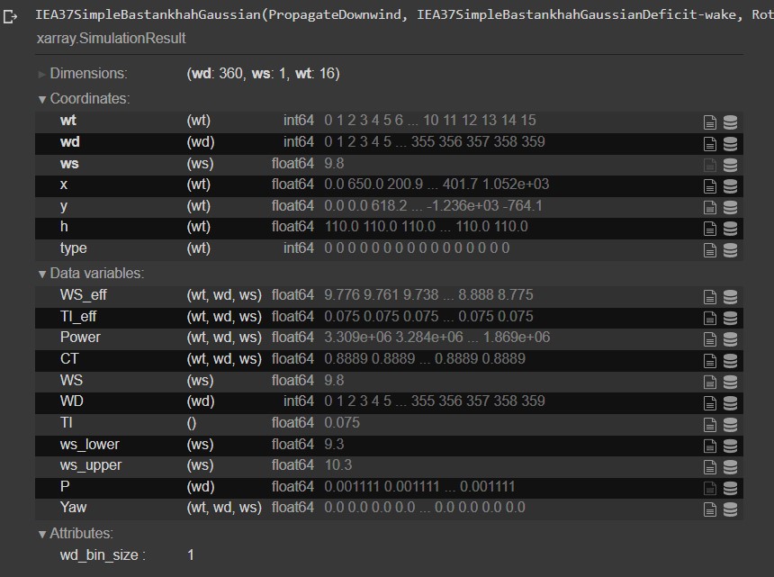
As you can see, the dataset returned by the simulation result has some co-ordinates such as :

wt: Wind Turbine Number.
wd: Ambient reference wind direction.
ws: Ambient reference wind speed
x, y, h : Represents position and hub height of wind turbines.

Besides that, it returns some of the data variables such as.

Wd: Local free-stream wind direction
Ws: Local free-stream wind speed
TI: Local free-stream turbulence intensity
P: Probability of flow case (wind direction and wind speed)
WS_eff: Effetive local wind speed [m/s] i.e. including wake effects.
TI_eff: Effective local turbulence intensity i.e. including wake effects.
power: Effective power production [W] i.e. including wake effects.
ct: Thrust coefficient
Yaw: Yaw misalignment [deg]

Conclusion

Today in this article, we have seen what AEP is and how to calculate it for a wind farm using Pywake Library in python. We have also seen how different factors affect the farm’s actual production. Then, we visualized the whole data using some plots. I hope this article has helped you. Thank you.