
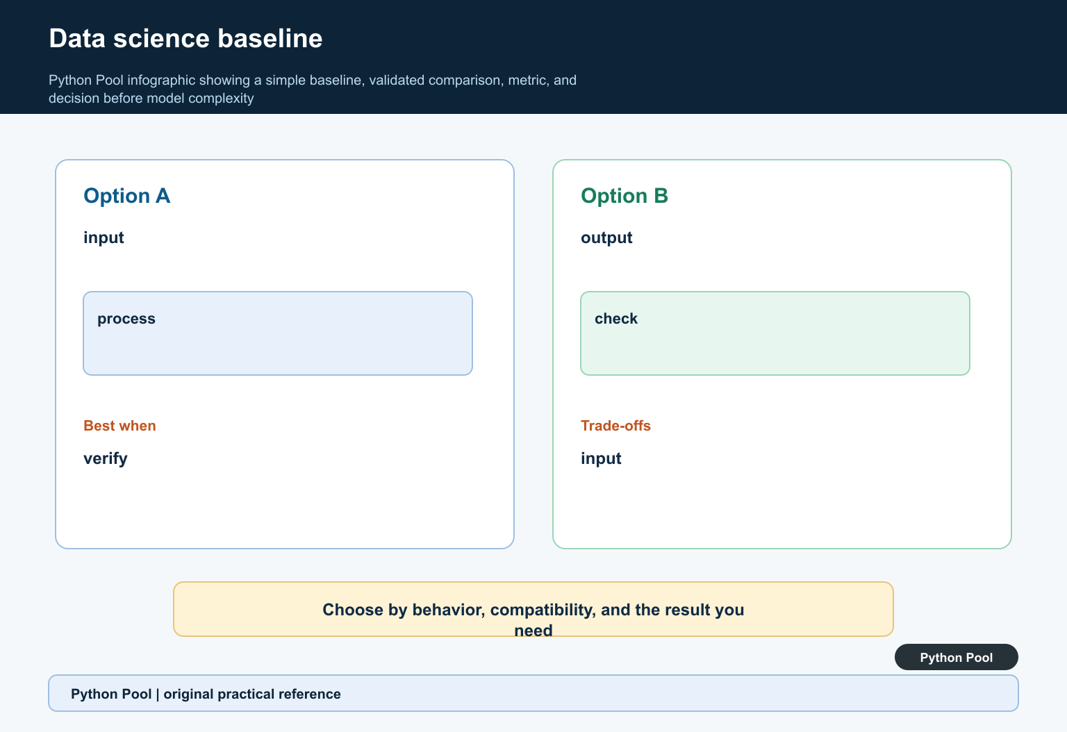
Quick answer: There is no universal top-ten algorithm list for data science. Start with the task and a simple baseline, inspect assumptions and data leakage, compare validated candidates, and include interpretability, cost, latency, and maintenance in the selection.
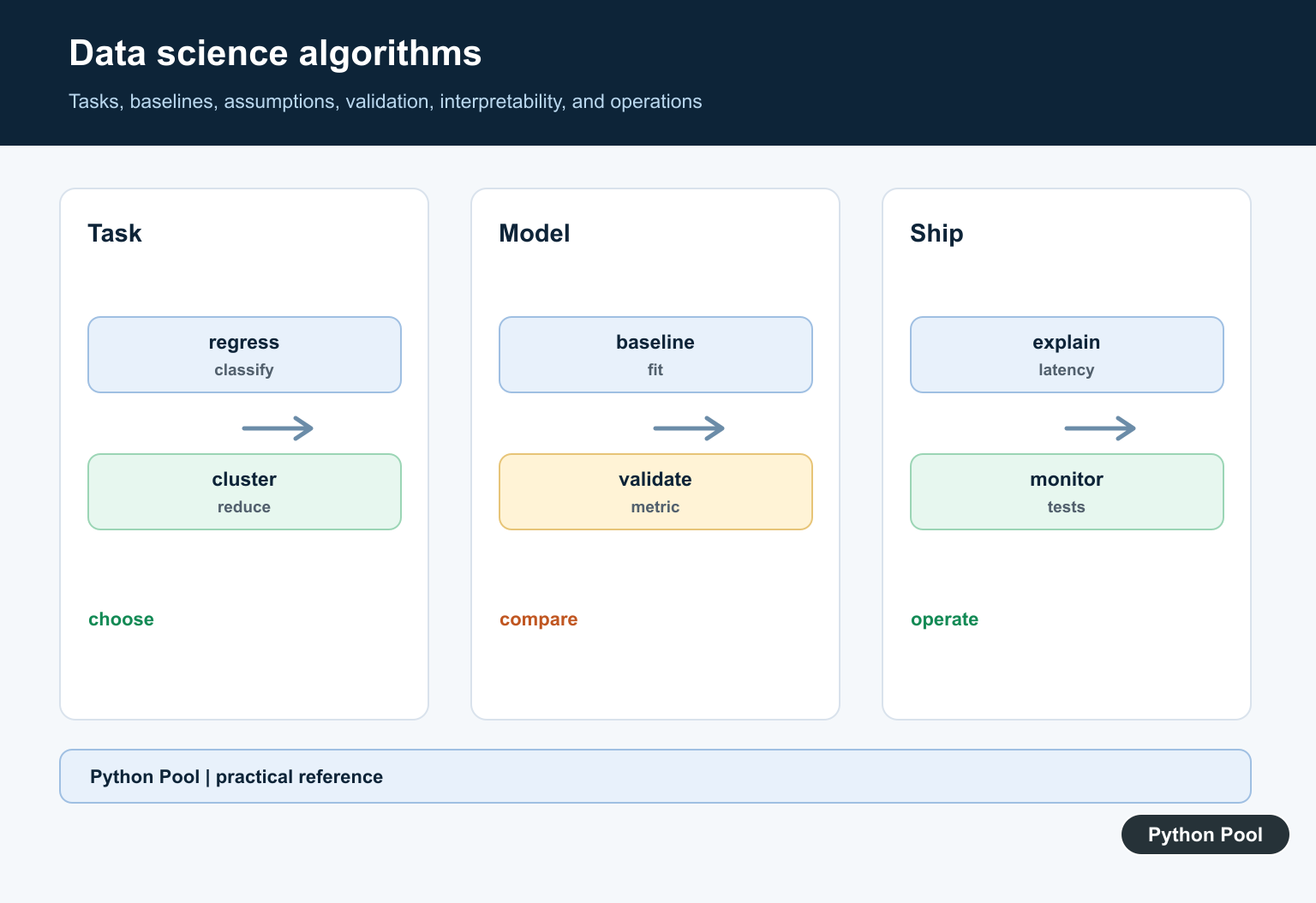
Algorithms for data science are not a ranked checklist. They are tools for different problem shapes: predicting numbers, classifying labels, finding groups, compressing features, or explaining a decision. The best Python workflow starts with clean data, a simple baseline, a validation split, and a model that matches the cost of being wrong.
This guide keeps the ten algorithms that are most useful for beginner and intermediate Python data science work: linear regression, logistic regression, decision trees, random forests, gradient boosting, support vector machines, k-nearest neighbors, Naive Bayes, K-means, and PCA. That list matches the way the scikit-learn user guide organizes supervised learning, unsupervised learning, preprocessing, and model evaluation. For decision-making agents beyond standard supervised and unsupervised algorithms, see the bounded AIXI experiments in AIXI Python: Toy Agents and Practical Limits.
The code examples are still useful because this is a Python article, but the code should not break the reading flow. The algorithm sections now focus on choosing the right method, while the runnable snippets are grouped later in a compact Python mini lab. For supporting data work, see PythonPool guides on CSV DictReader, NumPy arrays to pandas DataFrames, NumPy polyfit, averages in Python, and deep learning opportunities.
Quick Comparison Table
| Algorithm | Main Task | Best For | Needs Scaling? | Watch Out |
|---|---|---|---|---|
| Linear regression | Regression | Numeric targets and baselines | Sometimes | Outliers and nonlinear patterns |
| Logistic regression | Classification | Class probabilities and coefficients | Usually | Threshold and class imbalance |
| Decision tree | Classification or regression | Readable rules | No | Overfitting with deep trees |
| Random forest | Classification or regression | Strong tabular baseline | No | Less compact explanations |
| Gradient boosting | Classification or regression | High-performing tabular models | No | Tuning and validation leakage |
| Support vector machine | Classification | Margin-based separation | Yes | Large datasets and kernel choice |
| k-nearest neighbors | Classification or regression | Small local-pattern datasets | Yes | Slow prediction and noisy features |
| Naive Bayes | Classification | Text counts and fast baselines | No | Feature independence assumption |
| K-means | Clustering | Unlabeled grouping | Yes | Choosing k and interpreting clusters |
| PCA | Dimensionality reduction | Compression and visualization | Yes | Components can be hard to explain |
How To Choose A Data Science Algorithm
Start with the target. If the target is a number, try regression. If the target is a label, try classification. If there is no target, use clustering or dimensionality reduction. Then check the data shape: rows, columns, missing values, text, categories, and whether the features are on different scales. Finally, choose the metric before you fit anything. Accuracy, F1, ROC AUC, mean absolute error, and silhouette score answer different questions.
A practical order is simple: build a baseline first, then add complexity only when validation improves. Linear and logistic regression make strong first baselines. Trees and forests handle nonlinear tabular data. Boosting can improve accuracy when validation is strict. SVM and kNN need scaled features. Naive Bayes is a fast text baseline. K-means and PCA are useful when you are exploring unlabeled data.
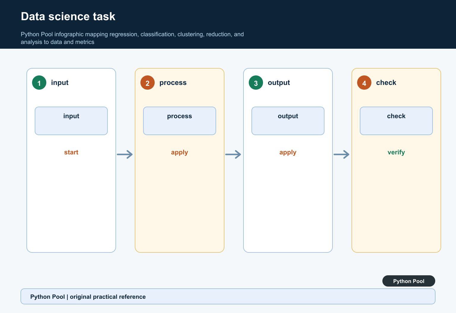
A Practical Python Workflow
For a real Python project, keep the workflow boring and repeatable. Load data, define the target, split rows, fit preprocessing on training data, train a baseline, choose a metric, and only then compare stronger algorithms. In scikit-learn, that usually means using estimators with the same fit(), predict(), and score() shape. That shared interface is why you can compare a linear model, a tree model, and a nearest-neighbor model without rewriting the whole project. For gradient-boosted regression where a skewed target needs transformation and inverse transformation, see CatBoostRegressor Target Transform Guide.
The best article or portfolio project does not simply say “I used random forest.” It says what the target was, which baseline it beat, which metric mattered, how the split was created, and which errors still remain. That evidence is what separates algorithm knowledge from copy-pasted model fitting.
Prepare Data Before Modeling
Most model failures begin before the algorithm. Parse fields intentionally, split train and test data before tuning, fit preprocessing only on training rows, and keep the target separate from the features. The official Python csv documentation and statistics module documentation are enough for small examples, while production work usually uses pandas, NumPy, and scikit-learn pipelines.
1. Linear Regression
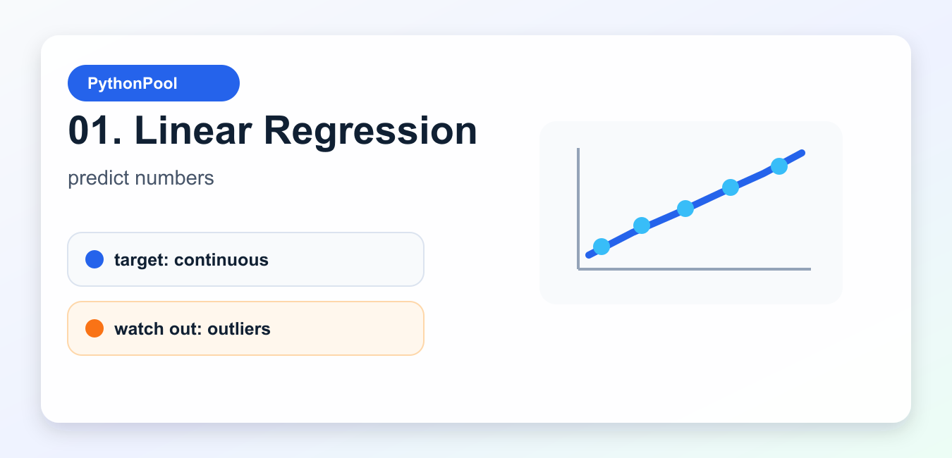
LinearRegression predicts a continuous value from one or more features. Use it for a transparent first model when the target is numeric: price, demand, duration, temperature, revenue, or error rate. It also gives you a baseline that more complex models must beat.
Do not treat linear regression as proof that the world is linear. Check residuals, outliers, and whether important interactions are missing. If the line is clearly wrong, try feature engineering, regularized linear models, trees, or gradient boosting.
2. Logistic Regression
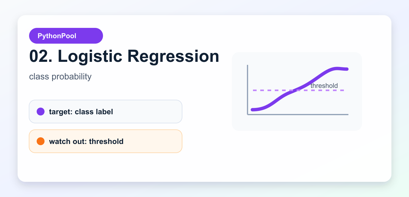
LogisticRegression is a classification algorithm despite the name. It estimates class probabilities, then a threshold turns those probabilities into labels. It is useful for churn prediction, fraud screening, moderation queues, and any problem where coefficients and probability calibration matter.
Scale numeric features, watch class imbalance, and choose the threshold from the business cost of false positives and false negatives. A default threshold is convenient, but it is not always the best decision rule.
3. Decision Trees
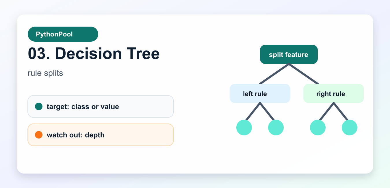
Decision trees split data into rule-like branches. They work for classification and regression, handle nonlinear patterns, and are easy to explain at shallow depth. They are excellent for teaching because every prediction follows a path of conditions.
The danger is memorization. Limit depth, require enough samples per leaf, and compare validation performance with a simpler baseline. If one tree is unstable, use a random forest or boosted trees.
4. Random Forests
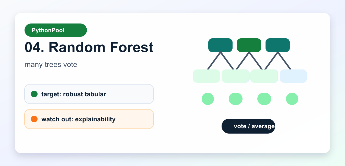
RandomForestClassifier and random forest regressors train many trees and combine their predictions. This reduces the instability of a single tree and often gives a strong tabular baseline with little preprocessing.
Random forests are good when you want accuracy, robustness, and feature importance hints. They are less compact than one tree, so explainability may need permutation importance, partial dependence, or a smaller surrogate model.
5. Gradient Boosting
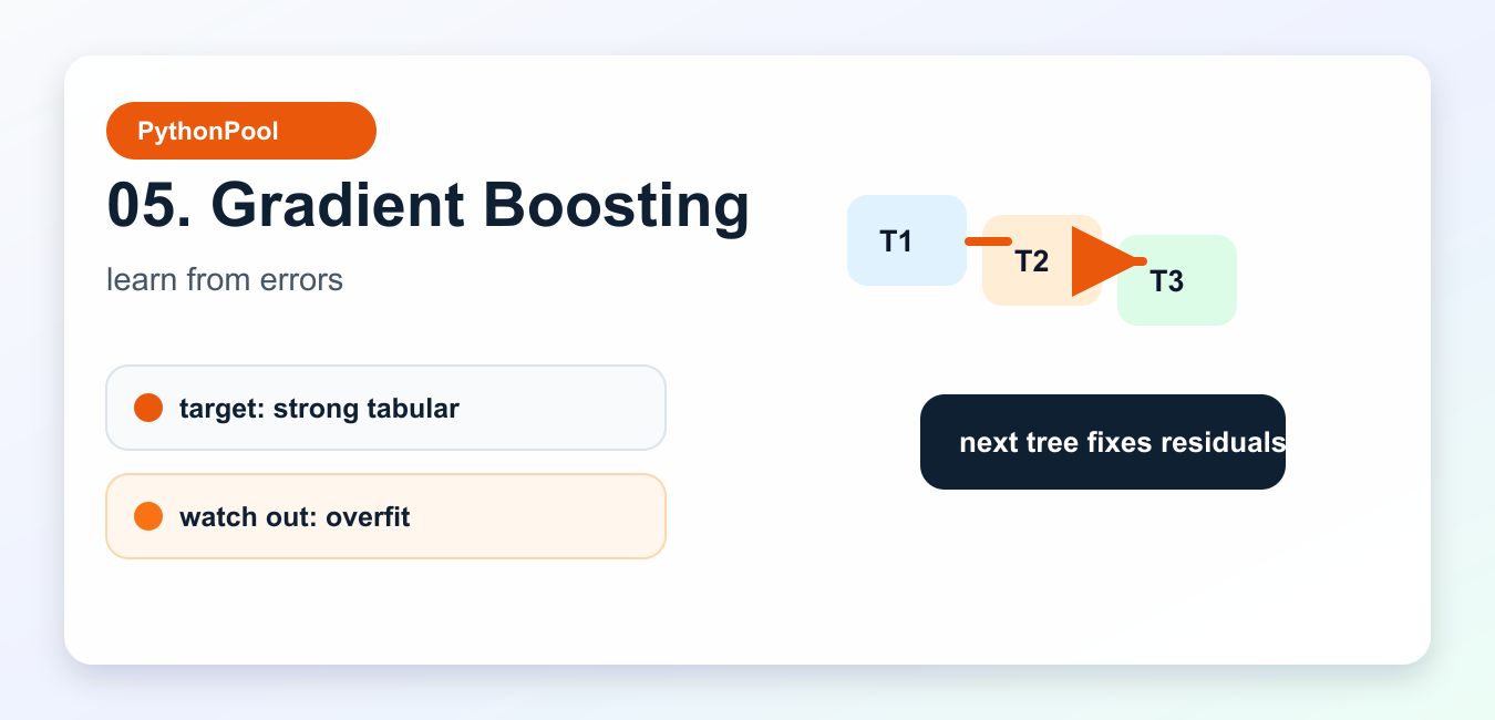
Gradient boosting builds trees sequentially, where each new tree focuses on the errors left by earlier trees. scikit-learn documents both classic gradient boosting and histogram-based gradient boosting in the ensemble methods guide. Boosted trees are often excellent for structured data.
The tradeoff is tuning. Learning rate, depth, iteration count, and early stopping all matter. Use a validation set or cross-validation, and avoid peeking at the test set while tuning.
6. Support Vector Machines

Support vector machines find a decision boundary with a wide margin between classes. Linear SVMs can be strong on high-dimensional text or sparse features, while kernel SVMs can model curved boundaries on smaller datasets.
SVMs are sensitive to feature scaling and hyperparameters. Try them when the dataset is not huge, the margin matters, and you can validate kernel and regularization settings carefully.
7. k-Nearest Neighbors
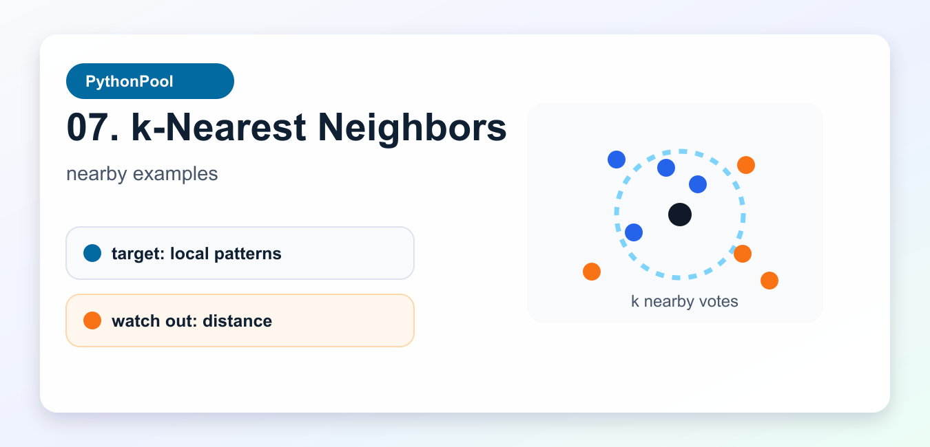
The nearest neighbors family predicts from nearby training samples. It is easy to understand and can work well when distance in feature space really means similarity.
kNN needs scaled features and careful feature selection. Prediction can become slow because the model compares new points to stored examples. It is a good learning tool, but not always the best production choice.
8. Naive Bayes
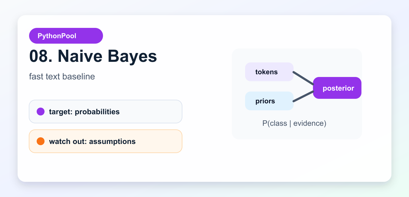
Naive Bayes uses Bayes’ theorem with a strong independence assumption. That assumption is rarely perfect, but the algorithm is fast and surprisingly useful for text classification, spam filters, ticket routing, and quick baselines.
Use it when features are counts or binary indicators and you need a fast reference model. If correlated features dominate the result, compare it with logistic regression or a linear SVM.
9. K-Means Clustering
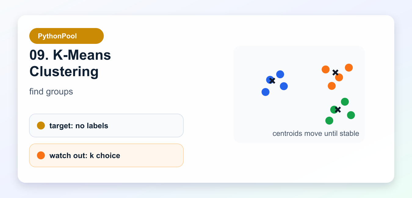
KMeans groups unlabeled points around centroids. It is useful for exploration, segmentation, compression, and finding rough structure before a supervised model exists.
The number of clusters is a design choice, not a discovered truth. Scale features, test several k values, inspect cluster stability, and decide whether the groups mean anything outside the model.
10. Principal Component Analysis
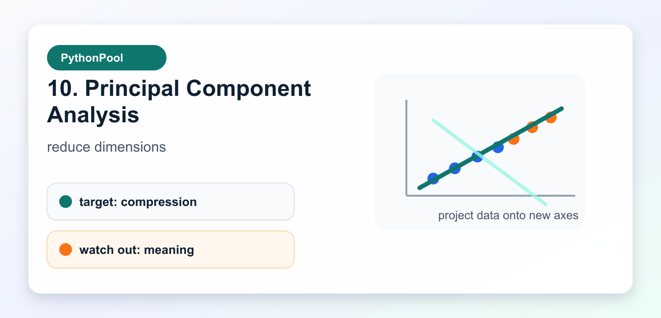
PCA projects centered data onto new axes that capture variance. It is useful for visualization, compression, denoising, and reducing many correlated features into fewer components.
PCA is not a classifier. It changes the feature space, so always evaluate the downstream model after transformation. Also remember that components are combinations of original features, which can make explanations harder.
Python Mini Lab
These short examples are here for technical readers who want executable anchors. They are intentionally standard-library examples, so the article stays runnable without installing heavy packages. For real projects, use scikit-learn estimators, pipelines, and metrics.
def fit_line(points):
    count = len(points)
    sum_x = sum(x for x, _ in points)
    sum_y = sum(y for _, y in points)
    sum_xx = sum(x * x for x, _ in points)
    sum_xy = sum(x * y for x, y in points)
    denominator = count * sum_xx - sum_x * sum_x
    slope = (count * sum_xy - sum_x * sum_y) / denominator
    intercept = (sum_y - slope * sum_x) / count
    return intercept, slope


model = fit_line([(1, 2.2), (2, 2.8), (3, 3.6), (4, 4.5)])
print(tuple(round(value, 3) for value in model))
from math import exp


def sigmoid(value):
    return 1 / (1 + exp(-value))


score = -1.2 + 0.8 * 3.0 - 0.4 * 2.0
probability = sigmoid(score)
label = int(probability >= 0.5)

print(round(probability, 3), label)
def tree_rule(row):
    if row["errors"] <= 2:
        return "ready"
    if row["hours"] >= 5:
        return "review"
    return "blocked"


ticket = {"hours": 6, "errors": 3}
print(tree_rule(ticket))
from collections import Counter
from math import dist

training = [((0.0, 0.0), "low"), ((0.2, 0.1), "low"), ((1.0, 1.1), "medium"), ((2.0, 2.2), "high")]


def knn_predict(rows, point, k=3):
    ranked = sorted((dist(point, features), label) for features, label in rows)
    votes = Counter(label for _, label in ranked[:k])
    return votes.most_common(1)[0][0]


print(knn_predict(training, (1.1, 1.0)))
from collections import Counter, defaultdict
from math import log

documents = [("refund invoice late", "billing"), ("invoice payment failed", "billing"), ("login password reset", "support")]
counts = defaultdict(Counter)
labels = Counter()
for text, label in documents:
    labels[label] += 1
    counts[label].update(text.split())

scores = {label: log(total / sum(labels.values())) + log((counts[label]["invoice"] + 1) / (sum(counts[label].values()) + 1)) for label, total in labels.items()}
print(max(scores, key=scores.get))
from math import dist

points = [(1.0, 1.0), (1.2, 0.8), (4.0, 4.0), (4.2, 3.8)]
centers = [(1.0, 1.0), (4.0, 4.0)]

groups = [[] for _ in centers]
for point in points:
    index = min(range(len(centers)), key=lambda i: dist(point, centers[i]))
    groups[index].append(point)

print([len(group) for group in groups])
Evaluation Metrics By Task
Pick the metric before comparing algorithms. Regression often uses mean absolute error or root mean squared error. Classification may use accuracy, precision, recall, F1, ROC AUC, or PR AUC depending on imbalance and cost. Clustering needs stability checks and domain review because there may be no true label. Dimensionality reduction should be judged by downstream task performance or how much structure it preserves.
Common Mistakes
The most common mistakes are fitting preprocessing on all rows before the split, choosing algorithms before defining the metric, trusting accuracy on imbalanced data, tuning on the test set, and treating unsupervised clusters as ground truth. A smaller model with honest validation is better than a complex model with leakage.
When Not To Use A More Complex Algorithm
Do not move to a complex algorithm just because it sounds more advanced. If the dataset is small, noisy, or poorly labeled, a stronger model may only memorize flaws. If the result must be explained to nontechnical people, a linear model or shallow tree may be more useful than a black-box ensemble. If the deployment environment is simple, a fast baseline can be easier to monitor and debug. For mathematical optimization with explicit decision variables and constraints rather than predictive modeling, continue with CPLEX Python and DOcplex Modeling Basics.
Complexity is justified when it improves the validation metric that matters and the team can still explain, reproduce, and maintain the workflow. That is why the comparison table matters: it gives you a reason to choose, not just a list to memorize.
Match The Task
Regression, classification, clustering, ranking, forecasting, dimensionality reduction, anomaly detection, and causal analysis require different objectives and evaluation designs.
Start With Baselines
A constant predictor, linear model, simple tree, or domain rule gives a reference point. Without a baseline, a complex model can look useful while adding little value.
Inspect Assumptions
Check scale, missing values, outliers, independence, linearity, class imbalance, stationarity, and feature leakage. Preprocessing must be fitted inside the appropriate training folds.
Compare Families
Trees and ensembles capture nonlinear interactions, linear models are interpretable, nearest neighbors depend on geometry, and clustering requires an appropriate similarity and validation story.
Validate Honestly
Use a split strategy that matches deployment, cross-validation where appropriate, task-specific metrics, uncertainty or calibration checks, and a held-out final evaluation.
Include Operations
Model size, prediction latency, retraining, explainability, monitoring, privacy, and dependency maintenance can outweigh a small offline metric improvement.
Use the official scikit-learn user guide for algorithm and evaluation details. Related Python Pool references include tests and array workflows.
For related data workflows, compare model tests, array preparation, and feature mappings before selecting an algorithm.
Frequently Asked Questions
Which algorithms are common in data science?
Linear and logistic regression, trees and ensembles, nearest neighbors, clustering, dimensionality reduction, gradient methods, and probabilistic models are common families.
How do I choose a data-science algorithm?
Start with the prediction or analysis task, create a baseline, inspect data and assumptions, compare validated candidates, and include interpretability and deployment constraints.
Why is validation important?
A model can fit training data while failing on new data; proper splits, cross-validation, leakage checks, and task-specific metrics estimate generalization.
Should I always use the most complex model?
No. A simpler model may be easier to validate, explain, deploy, and maintain while meeting the required performance.