CV2.findhomography: Things You Should Know

Hello coders!! In this article, we will be learning about cv2.findhomography in Python. But before getting into detail, let us get a basic idea about the topic.

What is homography?

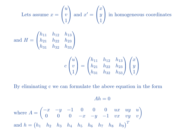
The homography is a 3×3 matrix that maps the points in one point to the corresponding point in another image. This matrix can be represented as:

If 2 points are not in the same plane, we have to use 2 homographs. Similarly, for n planes, we have to use n homographs.

Alignment of image using Homography

Let us consider a set of corresponding points (x1,y1) and (x2,y2). Then the Homography maps them in the following way:

The above equation is true for ALL sets of corresponding points, given that they lie on the same plane in the real world.

How to calculate a Homography?

To calculate the homography between two images, we must know at least four corresponding points between them. OpenCV robustly estimates a homography that fits all corresponding points in the best possible way. The point correspondences are found by matching features like SIFT or SURF between the images.

To calculate the homography between two images, we can use findhomography() method.

h, status = cv2.findHomography(points1, points2)

cv2.findhomography object tracking:

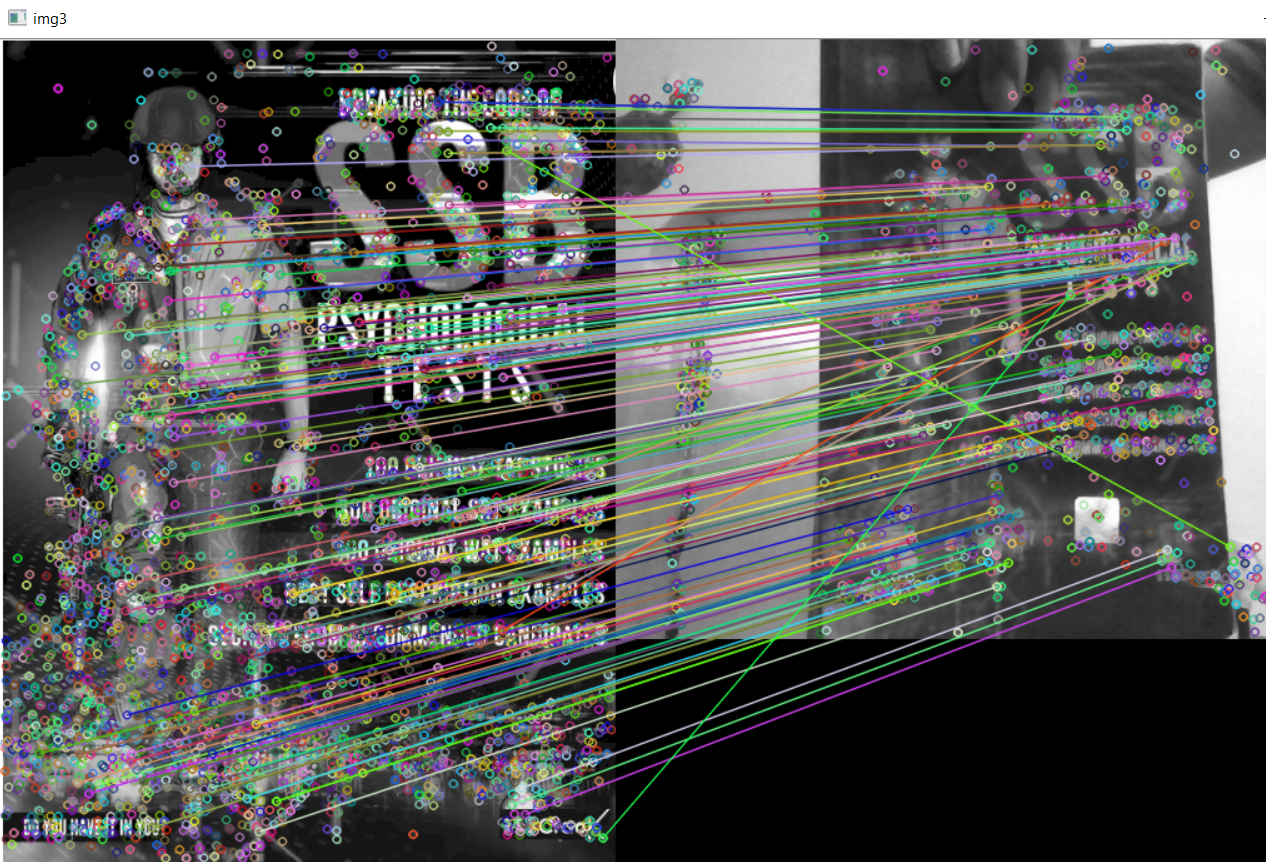
We will be using the following image for the understanding of cv2 homography:

import cv2 
import numpy as np 
img = cv2.imread("img.jpg", cv2.IMREAD_GRAYSCALE) 
cap = cv2.VideoCapture(0) 

Here, we have loaded the above image using the cv2.imread() method. We then use cv2.VideoCapture() method to initialize the webcam of the system.

Feature matching and homography to find objects:

Feature matching is the process of finding corresponding features from two similar datasets based on a search distance.

For this purpose, we will be using sift algorithm and flann type feature matching.

sift = cv2.xfeatures2d.SIFT_create() 
kp_image, desc_image =sift.detectAndCompute(img, None) 
index_params = dict(algorithm = 0, trees = 5) 
search_params = dict() 
flann = cv2.FlannBasedMatcher(index_params, search_params) 

In this code, we first created the SIFT algorithm using cv2.xfeatures2d.SIFT_create() method. We then found the keypoints and descriptors with SIFT using detectAndCompute(). After that, we initialized two dictionaries, index_params and search_params. Lastly, using flann type feature matching, we collected the two datasets’ corresponding features.

Now, we will convert the video capture into grayscale. 

_, frame = cap.read() 

grayframe = cv2.cvtColor(frame, cv2.COLOR_BGR2GRAY) 

kp_grayframe, desc_grayframe = sift.detectAndCompute(grayframe, None) 

matches= flann.knnMatch(desc_image, desc_grayframe, k=2) 
 
good_points=[] 

for m, n in matches: 
	
	if(m.distance < 0.6*n.distance): 
		good_points.append(m) 

Using cap.read(), we read the frame. We then convert this frame into grayscale using cvtColor(). Then we use SIFT to find the key points and descriptors. Using the KNN algorithm, we find the nearest match. We then initialize a list of good_points[] to keep track of only good points. Lastly, we use a for loop to append the points according to distance of descriptors.

Calculating homography using cv2.findhomography:

 
query_pts = np.float32([kp_image[m.queryIdx] 
				.pt for m in good_points]).reshape(-1, 1, 2) 

train_pts = np.float32([kp_grayframe[m.trainIdx] 
				.pt for m in good_points]).reshape(-1, 1, 2) 

matrix, mask = cv2.findHomography(query_pts, train_pts, cv2.RANSAC, 5.0) 

matches_mask = mask.ravel().tolist() 

h,w,d = img.shape

pts = np.float32([ [0,0],[0,h-1],[w-1,h-1],[w-1,0] ]).reshape(-1,1,2)

dst = cv.perspectiveTransform(pts, matrix)

homography = cv2.polylines(frame, [np.int32(dst)], True, (255, 0, 0), 3) 

cv2.imshow("Homography", homography) 

This code maintains a list of descriptors’ indexes in query descriptors and train descriptors. We then find the perspective transformation using cv2.findHomography. Mask.ravel() is used to get a contiguous flattened array. We then use cv2.polylines() to draw function for the frame. Lastly, we use cv2.imshow() to display the final output.

Conclusion| cv2.findhomography

With this, we come to an end with this article. I hope. You were able to grasp the concept of cv2 homography from this article.

However, if you have any doubts or questions, do let me know in the comment section below. I will try to help you as soon as possible.

Happy Pythoning!