
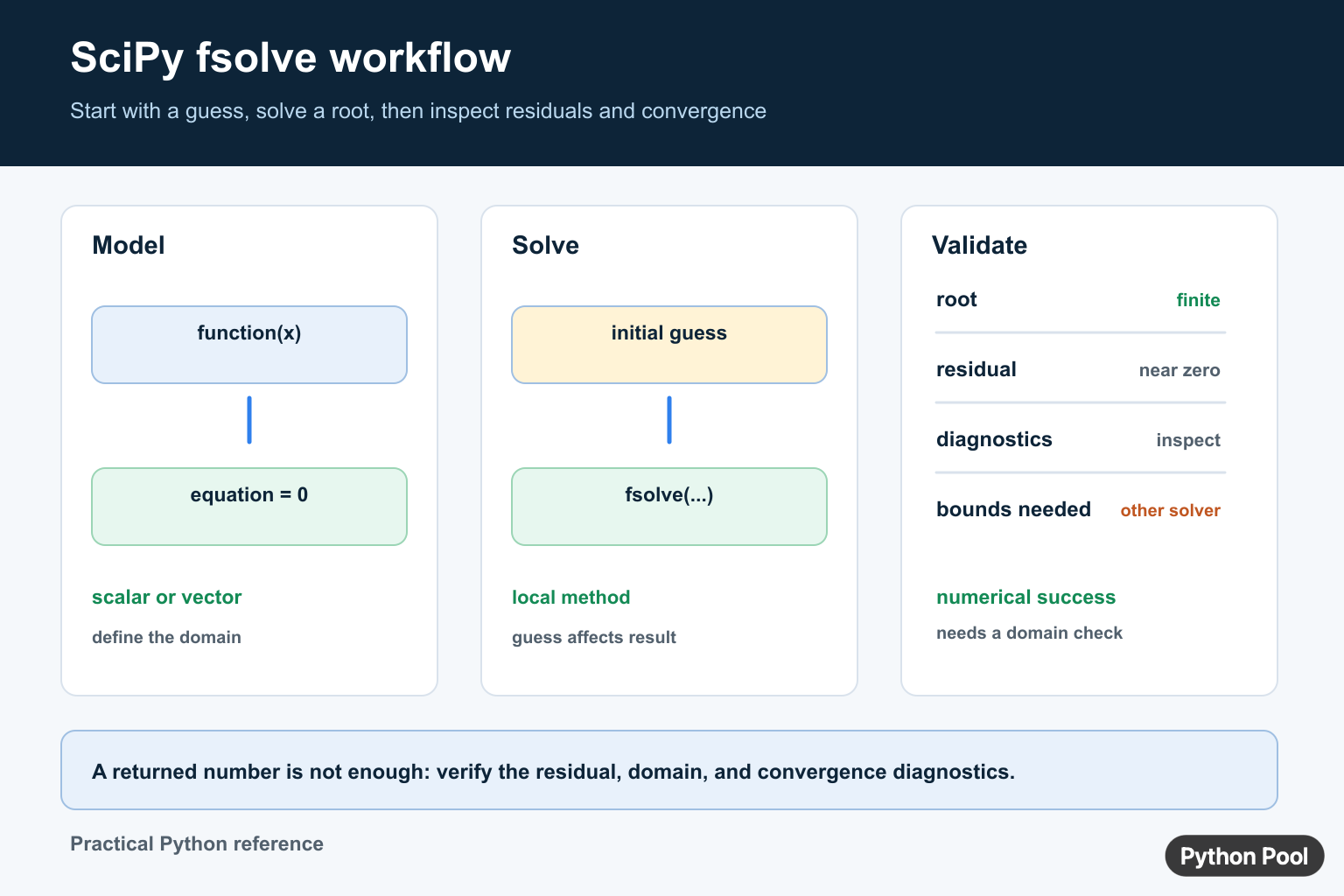
Quick answer: Use scipy.optimize.fsolve to find a root of a nonlinear equation or system from an initial guess. Always evaluate the residual at the returned value and inspect convergence diagnostics when the result matters.
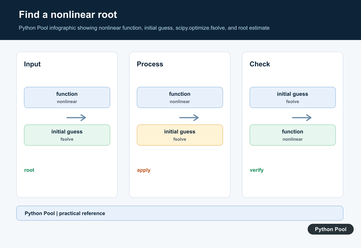
scipy.optimize.fsolve solves nonlinear equations by looking for inputs where a function returns zero. It is useful for scalar equations and for systems of equations when you can write the residuals as Python functions.
The official SciPy fsolve reference describes fsolve(func, x0, ...) as a root finder that starts from an estimate and returns roots for func(x) = 0. The broader scipy.optimize reference lists related root-finding tools such as root, root_scalar, brentq, and newton.
Use fsolve when your problem does not have a simple closed form and you can provide a reasonable starting estimate. It does not prove that every possible root was found. It follows the local shape near the estimate, so different starting points can return different roots.
The most common mistakes are passing a poor initial estimate, returning an output shape that does not match the input shape, ignoring the residual after the solve, and treating a returned number as correct without checking the convergence message.
Check Whether SciPy Is Installed
Before debugging a solver, confirm that the active Python environment can import SciPy.
try:
    import scipy
except ImportError as exc:
    print("SciPy is not installed:", exc.__class__.__name__)
else:
    print("SciPy", scipy.__version__)
If this prints an import error, install SciPy in the same environment that runs your code. In notebooks and IDEs, make sure the selected kernel or interpreter matches the terminal where you installed packages.
For reproducible work, store SciPy and NumPy versions in a dependency file. Solver behavior depends on floating-point libraries and package versions, so a pinned environment makes old results easier to reproduce.
Solve A Simple Equation
The equation x**2 - 9 = 0 has roots at -3 and 3. The starting estimate controls which root fsolve is likely to reach.
try:
    from scipy.optimize import fsolve
except ImportError:
    print("Install scipy to run fsolve")
else:
    def residual(x):
        return x[0] ** 2 - 9

    root = fsolve(residual, [2.0])
    print(round(float(root[0]), 6))
The residual function receives an array-like input, so this example uses x[0]. Returning a scalar for a one-equation problem is accepted, but for systems it is clearer to return one residual for each unknown.
Always choose a realistic starting estimate. If the function has multiple roots, start near the root you want, or scan the domain first and solve each bracketed area with a method better suited to scalar bracketing.
Check The Residual Yourself
A root is only useful if the function value at that point is close enough to zero for your problem.
def residual_at(x):
    return x * x - 9

candidate = 3.0
tolerance = 1e-8

print(abs(residual_at(candidate)) < tolerance)
print(residual_at(candidate))
This check should be part of your normal workflow. Floating-point solvers return approximate answers, and exact equality is the wrong test for most numerical results.
Use a tolerance that matches the scale of the problem. A residual of 1e-7 may be excellent in one model and unacceptable in another if units or downstream calculations are sensitive.

Solve A System Of Equations
fsolve can also solve systems when the function returns a list or array of residuals with the same length as the input.
try:
    from scipy.optimize import fsolve
except ImportError:
    print("Install scipy to run the system example")
else:
    def system(point):
        x, y = point
        return [x + y - 5, x - y - 1]

    root = fsolve(system, [1.0, 1.0])
    print([round(float(item), 6) for item in root])
For this system, the solution is near [3, 2]. If the returned residuals are not near zero, adjust the starting estimate, scale the equations, or switch to scipy.optimize.root for more explicit method choices.
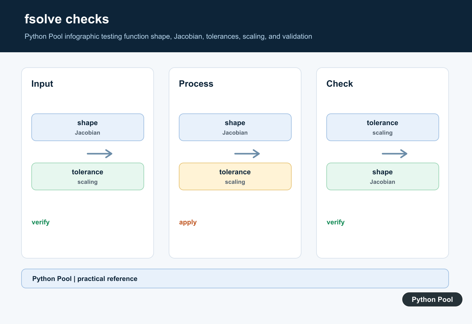
Shape matters. If you pass two unknowns, return two residuals. A mismatched shape usually indicates that the function definition needs to be rewritten before solver settings are adjusted.
Read The Solver Diagnostics
Use full_output=True when you need the convergence flag, message, and function-call count.
try:
    from scipy.optimize import fsolve
except ImportError:
    print("Install scipy to inspect full_output")
else:
    def residual(x):
        return x[0] ** 2 - 9

    root, info, flag, message = fsolve(residual, [2.0], full_output=True)
    print(round(float(root[0]), 6))
    print(flag == 1)
    print(info["nfev"] > 0)
In SciPy’s API, a success flag of 1 means a solution was found. Other flags should be treated as warnings that the returned value may be only the last attempted iterate.
The message often tells you whether the solver struggled with progress, maximum calls, or tolerance. That is more informative than only printing the root.

Choose The Right Root Finder
fsolve is not always the best tool. For scalar functions with a known sign change, a bracketing method can be more reliable.
choices = [
    ("single equation with bracket", "root_scalar or brentq"),
    ("system with starting estimate", "fsolve or root"),
    ("least-squares residuals", "least_squares"),
    ("needs bounds", "least_squares or minimize"),
]

for situation, solver in choices:
    print(f"{situation}: {solver}")
If the equation has discontinuities, flat areas, or roots far from the starting estimate, no solver setting can fully replace understanding the function. Plot or sample the residual first when results look surprising.
In short, write a residual function, choose a realistic starting estimate, run fsolve, inspect the residual and convergence flag, then compare with other SciPy root finders if the problem needs bracketing, bounds, or more method control.
Choose An Initial Guess Carefully
fsolve() is a local numerical solver. It starts from the guess you provide, so different guesses may converge to different roots, fail to converge, or reach a point that is not useful for your problem. Try a small set of reasonable guesses when the equation may have multiple solutions.
import numpy as np
from scipy.optimize import fsolve

def equation(x):
    return x**2 - 4

for guess in (-3.0, 3.0):
    root = fsolve(equation, guess)[0]
    print(root, equation(root))
Validate More Than The Root Value
A small-looking root is not enough evidence. Check the residual, finiteness, expected domain, and convergence flag. Scale variables when one component is much larger than another, and use bounds or a different solver when the solution must stay inside a known interval.
For a single scalar equation with a bracket, a bracketing method can provide a stronger guarantee. For least-squares problems, constraints, or systems with special structure, choose the solver family from the mathematical contract rather than defaulting to fsolve.
For numerical solving, compare fsolve() diagnostics with singular-matrix checks and summaries. Read linalgerror singular matrix and numpy mean for the related workflow.
Frequently Asked Questions
What does scipy.optimize.fsolve() do?
fsolve() searches for a root of a nonlinear equation or system from an initial estimate supplied by the caller.
Why does fsolve() need an initial guess?
It is a local numerical method, so the initial guess influences which root it approaches and whether it converges.
How do I check whether fsolve() succeeded?
Evaluate the residual at the returned solution and inspect the convergence flag and diagnostic message when using full_output=True.
When should I use another SciPy root solver?
Use a bracketing method when you have a valid interval, or another solver when you need bounds, constraints, or a different numerical contract.