Moving Average Python | Tool for Time Series data

Moving Average in Python is a convenient tool that helps smooth out our data based on variations. In sectors such as science, economics, and finance, Moving Average is widely used in Python. In a layman’s language, Moving Average in Python is a tool that calculates the average of different subsets of a dataset.

Contents

Introduction – Time-series Dataset and moving average

A time-series dataset is a dataset that consists of data that has been collected over time in chronological order. It is assembled over a successive time duration to predict future values based on current data. Time series consist of real values and continuous data. The stock market, weather prediction, sales forecasting are some areas of application for time series data. With the help of moving average, we remove random variations from the data, thus reducing noise.

TYPES OF MOVING AVERAGE

There are many different types of moving averages but the main types are :

Simple Moving Average (SMA)
Exponential Moving Average (EMA)
Cumulative Moving Average (CMA)

1. Simple Moving Average (SMA)

Simple Moving Average is the most common type of average used. In SMA, we perform a summation of recent data points and divide them by the time period. The higher the value of the sliding width, the more the data smoothens out, but a tremendous value might lead to a decrease in inaccuracy. To calculate SMA, we use pandas.Series.rolling() method.

2. Exponential Moving Average (EMA)

EMA focuses more on recent data by assigning more weight to new data. The main idea behind EMA is to give preference to the recent data more than previous data. The older the data, the lesser is the weight assigned to it. Because of this, the EMA is more responsive to changes in trend compared to SMA, where all values are given equal weights. To calculate EMA, we use pandas.Series.ewm() method.

3. Cumulative Moving Average (CMA)

Cumulative Moving Average is the mean of all the data up to a current time ‘t.’ Like SMA, and it is unweighted mean, i.e., all the values are assigned equal weights. But unlike SMA, which has a constant window size, in CMA, the width of the window increases as duration increases. To calculate CMA, we use pandas.Series.expanding() method.

SEMANTICS

Before we jump into coding, let us understand how it works. The main idea behind finding average is to smooth out variations to highlight the hidden patterns in data. A line represents it on a chart. Next, we have to specify a window width for how many data points we have to calculate the average for a time. The word ‘moving’ word itself suggests that we have to slide the window width for every new set of values.

For example: Let us take a list named ‘dataset’ and assign it some values.

dataset = [4,9,2,7,4]

If the window size is 3, then we shall take 3 values to calculate their average and move to the next three values.

First, we shall calculate the average (4,9,2), which is (4+9+2)/3 = 5. Then for the next three values, we shall take (9,2,7), which is (9+2+7)/3 = 6, and so on.

Let us understand by taking a more concrete example.

EXAMPLE OF MOVING VALUES USING PANDAS

Pandas is an open-source python library that is used for data analysis. First, we shall import pandas

import pandas as pd

The dataset used here is a sales dataset. A snippet of dataset if given below.

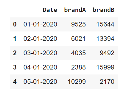
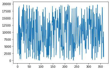
Now, we shall plot the column ‘brandA’

df['brandA'].plot()

It plots all the sales values as given below.

Similarly, we plot the values for the column ‘brandB’ also.

df['brandB'].plot()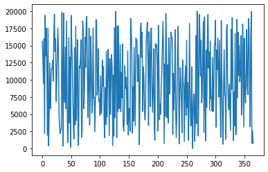

As seen in both cases, there is a lot of variation present in the data. Because of the variations present, we shall use pandas.DataFrame.rolling function to smoothen it out. It is used for rolling window calculations. We shall calculate the moving average for ‘brandA.’ The rolling function shall group the observations on the window width chosen.

Here, we are setting the window width to 20.

df['brandA'].rolling(window =20).mean().plot()

As the output, we get our rolling average.

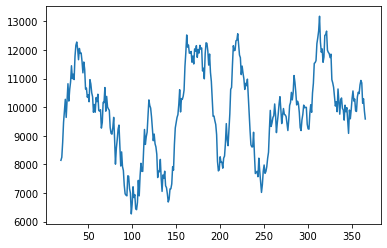
To better understand the moving average, we shall plot both the original dataset and the rolled dataset together.

df['brandA'].plot(figsize=(10,6))
df['brandA'].rolling(window =20).mean().plot()

The yellow line plotted below, is our moving average line.

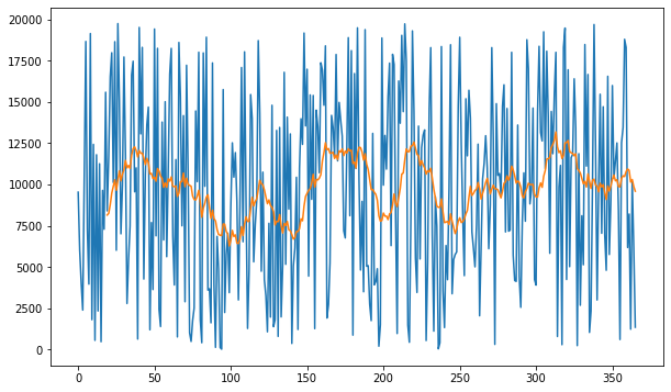
We can clearly see through the above-given graph that the rolling average has smoothened out the sales graph.

Now, we shall create a new column named ‘moving_avg’ to reflect the changes on our dataset.

df['moving_avg'] = df['brandA'].rolling(window=20).mean()
df.head(30)

Here we shall display the first 30 rows of our dataframe.

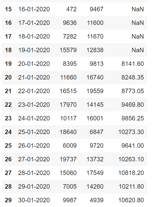
As given above, we can see that the first few observations had to be discarded.

Also, Read

SUMMARY

In this article, we covered :

Time Series data with moving average
Types of moving average
Understanding the semantics behind the code
Took a sample dataset and learned how to implement moving average using rolling() function