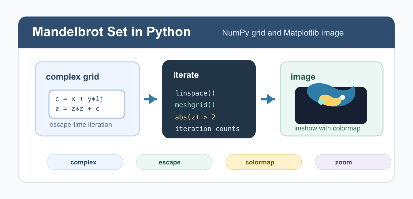
Mandelbrot Set in Python: Complex Iteration and Visualization

Quick answer: Generate the Mandelbrot set by iterating z = z² + c from z = 0 across a complex grid and recording whether each point escapes the chosen radius within an iteration limit. Resolution, iterations, coloring, and performance all affect the image.

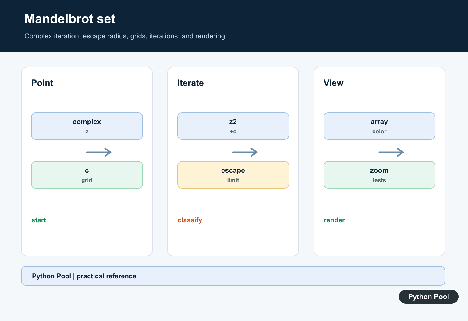
Python Pool infographic showing complex points iterated through z squared plus c and classified by whether they escape a radius — The Mandelbrot calculation iterates z = z² + c for each complex point and records whether the magnitude escapes the chosen limit within the iteration budget.

The Mandelbrot set is generated by repeatedly applying z = z * z + c to points on the complex plane. A point belongs to the set when the sequence does not escape to infinity. In code, we usually draw the set with an escape-time algorithm: count how many iterations each point takes to move beyond a radius of 2.

Python can generate a Mandelbrot image with plain loops, but NumPy makes it much faster by evaluating many complex numbers at once. Matplotlib then turns the iteration-count array into an image with imshow().

The resulting picture is not a random drawing. Every pixel represents a complex number, and the color represents how quickly that number escaped. Points that never escape within the iteration limit are usually colored as the inside of the set.

Test One Complex Point

Start with one complex number. If the absolute value of z becomes greater than 2, the point has escaped. The iteration number gives a useful color value.

def mandelbrot_point(c, max_iter=50):
    z = 0j
    for iteration in range(max_iter):
        z = z * z + c
        if abs(z) > 2:
            return iteration
    return max_iter

print(mandelbrot_point(complex(-0.75, 0.1)))

This function is easy to understand, but calling it for every pixel with Python loops can be slow. The same idea scales better when the whole image is represented as NumPy arrays. Keeping this simple version around is still useful for explaining and testing the algorithm.

Create a Complex Grid With NumPy

A Mandelbrot image needs a rectangular grid of complex coordinates. Use np.linspace() for the x and y ranges, then np.meshgrid() to combine them.

import numpy as np

width, height = 800, 500
x = np.linspace(-2.0, 1.0, width)
y = np.linspace(-1.2, 1.2, height)
X, Y = np.meshgrid(x, y)
C = X + 1j * Y

print(C.shape)

The array C contains one complex value per pixel. For more on vectorized numeric arrays, see Python vectors with NumPy and NumPy ogrid. The grid limits control the part of the fractal you see.

Compute Escape Iterations

Now iterate over the whole grid. Track which points are still active, update only those points, and store the iteration where each point escapes.

import numpy as np

Z = np.zeros_like(C)
escape = np.full(C.shape, 100, dtype=int)
active = np.ones(C.shape, dtype=bool)

for iteration in range(100):
    Z[active] = Z[active] * Z[active] + C[active]
    escaped = np.abs(Z) > 2
    newly_escaped = escaped & active
    escape[newly_escaped] = iteration
    active &= ~escaped

print(escape.min(), escape.max())

The escape array is the image data. Low values escaped quickly, while high values stayed bounded for longer. The maximum iteration count controls detail and runtime. Updating only active points avoids wasting work on coordinates that already escaped.

Python Pool infographic showing a complex coordinate, real and imaginary axes, and Mandelbrot input — Complex plane: A complex coordinate, real and imaginary axes, and Mandelbrot input.

Display the Mandelbrot Set

Use Matplotlib imshow() to display the escape-count array. The extent argument maps image coordinates back to the complex-plane range.

import matplotlib.pyplot as plt

plt.imshow(
    escape,
    extent=[x.min(), x.max(), y.min(), y.max()],
    origin="lower",
    cmap="magma",
)
plt.xlabel("Real")
plt.ylabel("Imaginary")
plt.title("Mandelbrot set")
plt.colorbar(label="Iterations")
plt.show()

Changing the colormap changes the mood of the image without changing the math. See Matplotlib imshow() and custom Matplotlib colormaps for more display options.

Save the Image

For scripts, save the generated image instead of only showing it interactively. plt.imsave() writes the array with the selected colormap.

import matplotlib.pyplot as plt

plt.imsave("mandelbrot.png", escape, cmap="magma", origin="lower")
print("saved mandelbrot.png")

Saving the raw iteration array separately can also be useful if you want to experiment with different colormaps later without recomputing the fractal. For repeatable output, keep the width, height, limits, and iteration count in variables at the top of the script.

Zoom Into a Region

Zooming is done by narrowing the x and y ranges and recomputing the grid. Smaller ranges usually need more iterations to reveal detail.

x = np.linspace(-0.8, -0.7, width)
y = np.linspace(0.05, 0.15, height)
X, Y = np.meshgrid(x, y)
C = X + 1j * Y

print(C.real.min(), C.real.max())
print(C.imag.min(), C.imag.max())

Use a higher max_iter for deeper zooms. Otherwise many points may hit the iteration cap and the image will look flat. If the zoomed region looks empty, widen the coordinate range or start from a known interesting boundary area.

Python Pool infographic mapping z through z squared plus c, iteration count, escape radius, and membership — Escape iteration: Z through z squared plus c, iteration count, escape radius, and membership.

Balance Quality and Speed

Image size and iteration count are the two main performance knobs. Doubling width and height creates four times as many pixels, and increasing max_iter adds more work for each active point. Start with a small image while tuning the coordinate range, then increase resolution for the final render.

Common Mistakes

The most common mistake is using too few iterations for a detailed zoom. Another is forgetting origin="lower", which flips the image vertically compared with the complex plane. A third is recomputing points that already escaped, which wastes time on large images.

Use NumPy arrays for speed, keep the complex-plane limits explicit, and separate calculation from rendering. That makes it easy to change image size, colormap, and zoom region without rewriting the Mandelbrot logic. For large images, increase resolution gradually so you can see the runtime cost before committing to a huge render.

Python Pool infographic showing a pixel grid, complex coordinates, iteration count, color map, and image — Render set: A pixel grid, complex coordinates, iteration count, color map, and image.

References

Create A Complex Grid

Choose real and imaginary bounds and map pixels to complex values. Keep the coordinate convention explicit so zooming and aspect ratio do not distort the set.

Apply The Escape Rule

For each c, start z at zero and iterate z*z + c. Once the magnitude exceeds the escape radius, the point is classified as escaping; points that remain bounded through the limit are retained as interior candidates.

Choose Resolution And Iterations

More pixels increase spatial detail and more iterations improve boundary classification. Use small previews while tuning the view, then scale the expensive calculation for the final output.

Python Pool infographic testing bounds, max iterations, precision, zoom, and performance — Fractal checks: Bounds, max iterations, precision, zoom, and performance.

Color The Boundary

The iteration count can drive a gradient or discrete palette. Keep the color mapping separate from the classification array so the mathematical result can be reused for different visual styles.

Improve Performance

Vectorized NumPy operations can process a grid efficiently, but memory use grows with resolution. Profile before choosing chunking, compiled loops, or parallel execution, and keep numerical overflow behavior in mind.

Test Known Behavior

Test a small grid, symmetric coordinates, bounded interior points, obvious escaping points, zoom windows, iteration changes, and saved image dimensions. Verify that axes and orientation are documented.

Use the official NumPy broadcasting guide when vectorizing grid operations. Related Python Pool references include NumPy arrays and tests.

For related numerical visualization, compare grid arrays, calculation tests, and sequence iteration before rendering the Mandelbrot set.

Frequently Asked Questions

What is the Mandelbrot set?

It is the set of complex numbers c for which iterating z = z² + c from z = 0 does not escape under the chosen mathematical definition.

How do I plot the Mandelbrot set in Python?

Create a complex grid, iterate each point up to a limit, record escape information, and render the resulting array with a plotting library.

Why do image resolution and iterations matter?

Resolution controls spatial detail, while the iteration limit controls how confidently boundary points are classified; both increase computation cost.

How can I speed up a Mandelbrot calculation?

Use vectorized NumPy operations, compiled numerical code, or carefully managed parallelism, and profile before changing the algorithm.